New Zealand general election forecasts - state space model
Introducing “Model B”
This page provides an estimate of New Zealand election probabilities that feels even slightly more experimental than my Model A and predictions. This method is called a state space model. It models the latent voting intention for each party, and the biases of polling house effects, simultaneously, drawing on the 2011 and 2014 election results and all polls since 2011. The approach aims to apply to a multi-party proportional representation system a modelling approach set out by Simon Jackman in a key 2005 article in the Australian Journal of Political Science, Pooling the Polls Over an Election Campaign.
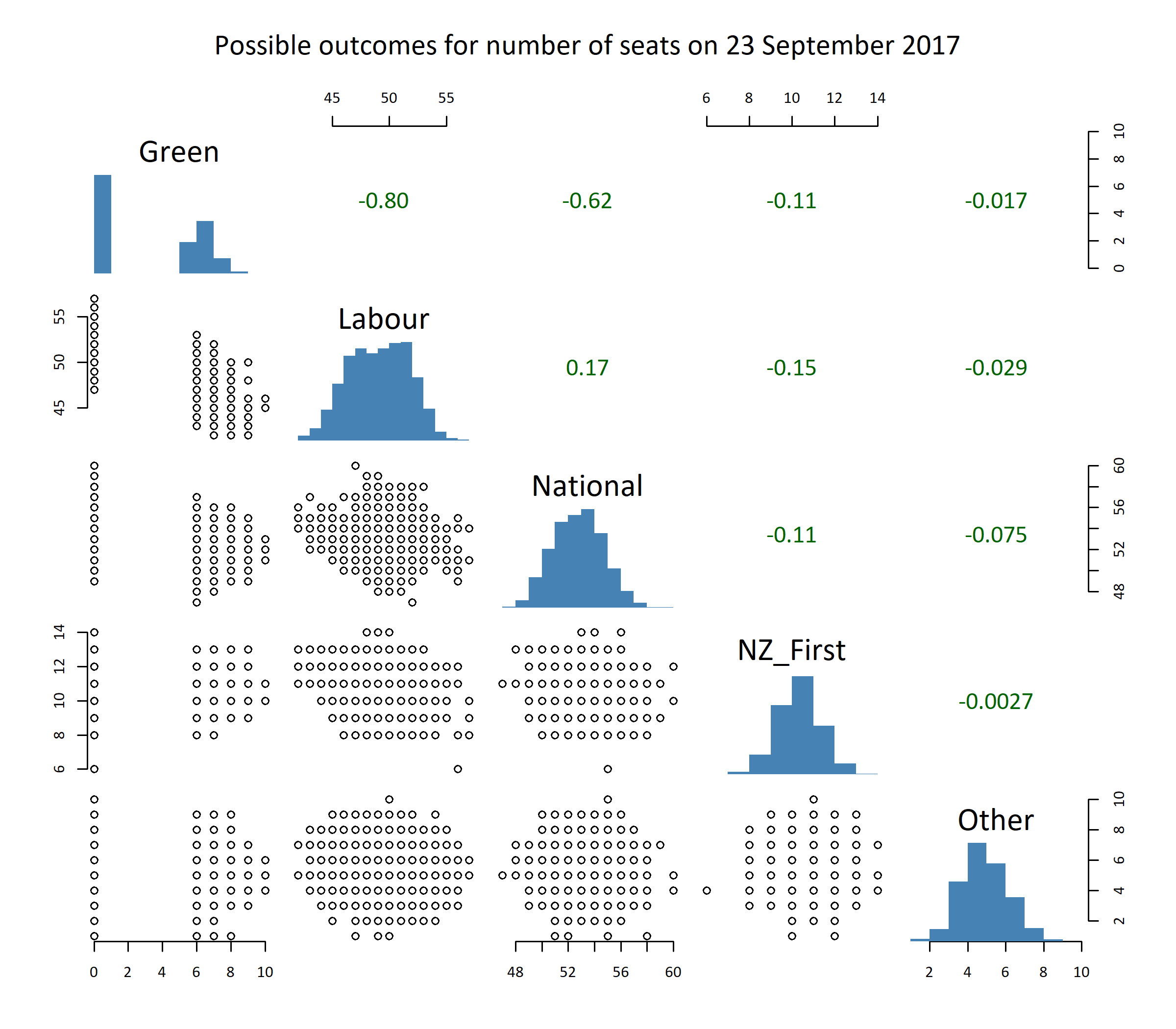
Results
Treat these results with caution, the recommended approach is the combination of my two models.


Differences in method
The two modelling approaches have different ways of estimating party vote for each party on election day. The conversion of party vote to seats, including the assumptions for key electorate seats that might lead to parties with less than 5% of the party vote still getting into Parliament, are the same.
With the differences that have most implications for results listed at the top, here are the substantive differences between these two methods for forecasting party vote:
Random walk rather than structural change
The state space model assumes that underlying voting intent is a random walk. This means that regardless of the path taken in voting intent getting to a certain point, from that point it is as likely to go up as down. In contrast, the generalized additive model behind the main set of election predictions implicitly assumes some underlying structural change; if the vote for a party has been steadily growing for a few years (as is currently the case for New Zealand First), it models that growth to continue rather than to stablise at the current point.
This feature can be seen by looking at the graphic below, and comparing it to a similar chart on the page with the generalized additive model’s results:

Only data from 2011 onwards used for house effects
The state space model only uses polling data subsequent to the 2011 election in its estimation of house effects, whereas the generalized additive model uses data all the way back to 2002. This is for three reasons:
- Mostly it is a matter of practicality. The state space model (partly due no doubt to my non-optimal Stan programming skills) takes more than an hour to converge with just two election cycles of days to estimate and this length of time would increase materially with further days.
- There is a also plausible assumption that house effects from 2008 and before are not particularly relevant for 2017. Polling firms constantly try to fix the problems behind biases.
- The generalized additive model needs to use multiple election years to get any statistical sense of the house effects, whereas systematic Bayesian approach used in the state space model means even one election result would be enough to get meaningful estimates (so using both 2011 and 2014 is a bonus).
Here are the estimated house effects from the state space model:

For Reid Research, there is an additional 2017 house effect on top of the “2016 and earlier” effect shown above. See this blog post for more discussion - the long and short of it is that National look to be a bit overstated and Labour understated in Reid Research polls in 2017, compared to the house effect in 2016 and earlier.
Everything modelled together rather than ad hoc
The generalized additive model I use for Model A has a somewhat ad hoc, thrown together feel. First the house effects are estimated by fitting models to previous years and comparing with election results. Then “election day variance” is estimated similarly. Finally a model is fit to the current cycle’s polls, adjusted with those house effects, used to project forward to election day with election day variance added; and simulations created based on this combination.
In contrast, these components are satisfyingly combined in a single model in the state space approach. The house effects are estimated at the same time as the latent voting intention for six parties and “other” for every day; the voting intention right up to election day is estimated at the same time, not in a separate election process; and all the sources of variance are driven from the model without having to be estimated separately and added in. Everything is held together by Bayes’ rule. Then, even the simulations at the end come as a by product of the model-fitting in Stan.
Why isn’t Model B used by itself rather than in combination with Model A?
The state space model is much more satisfying for a statistician than the more ad hoc approach in Model A, and I think maybe in a future year will be my main model. But for now, I’m not letting it dominate, because:
- It’s still experimental and I’m tweaking with it. For example, on the day I released the model I respecified the whole thing so that the day to day innovations in latent voting intention for each party are correlated with eachother rather than independent as had been the case before. This is just playing catchup with the Model A, which has treated latent vote as multivariate normal on the logit scale since well before I began publishing it. I have a list of other improvements in my head (which I may or may not get around to before election day in September), and I don’t know in advance how much they might impact on the result. So I don’t want to be highlighting its predictions.
- I’m twitchy about the random walk assumption. In fact, I’m pretty sure it’s just plain wrong; there’s good evidence that in fact latent voting intention converges systematically towards levels that would be predicted by non-polling political science models. See for example this great article Understanding Persuasion and Activation in Presidential Campaigns: The Random Walk and Mean-Reversion Models by Kaplan, Park and Gelman. Of course, my simplistic generalized additive model isn’t necessarily picking up structural reversion to an underlying destination better; but at least it’s got a fighting chance.
My preferred model would be one that uses a political science prediction of the result (based on incumbency length, unemployment, etc) as a prior, and then the polling data updates that prior. Alternatively (or in addition), I could just use splines in Stan instead of random walks for the underlying voting intention, thereby combining the approaches of the two. But I haven’t got around to either of these yet and may not get to it. There would certainly be costs and risks associated with either.
The closer we get to election day, the less it matters. This is because the main difference between the two models is the prediction of what happens between now and election day. The state space model effectively treats recent polls (after treating for house effects) as a straight indication of the election day result; the generalized additive model instead expects there to continue to be movement in the current direction in the remaining days. As the remaining days gets fewer this makes no difference, and I expect the two models to converge.
In the meantime I recommend that you use the combination of both models. A substantial literature in forecasting shows that when you have two reasonably good models, you often get closer results by combining the two, so I’ve done this for you.
Source code
All the source code for both models is available in my nz-election-forecast GitHub repository. The guts of the model is in the file ss-vectorized.stan, but all the data management, munging and presentation of results is in R. Start with the integrate.R file to get a sense of how it hands together.