Motivation
This post is the fourth in a series that make up my entry in Ari Lamstein’s R Election Analysis Contest.
Earlier posts introduced the nzelect R package, basic usage, how it was built, and an exploratory Shiny web application. Today I follow up on discussion in the StatsChat blog. A post there showed a screen shot from my Shiny app, zooming in on Auckland votes for Green Party compared to the Labour Party (the two principal left-leaning parties in New Zealand). There was discussion in the comments of whether house price, income, and education were the predictors of the choice between these two parties (for the subset of voters who chose one of the two).
Combining census meshblock data with voting locations
Making it easier to investigate this issue is one the primary motivations for the nzelect R package and incorporating census data that can be matched to voting locations and electorates has been on the plan from the beginning. It’s proven a bigger job than I hoped and is very incomplete, but so far I’ve incorporated around 35 selected variables from the 2013 Census at the meshblock level.
First look
The plot below shows how some of those variables relate to the variable of interest here - the Green Party votes as a proportion of all that went to Green Party or Labour Party, by voting location.
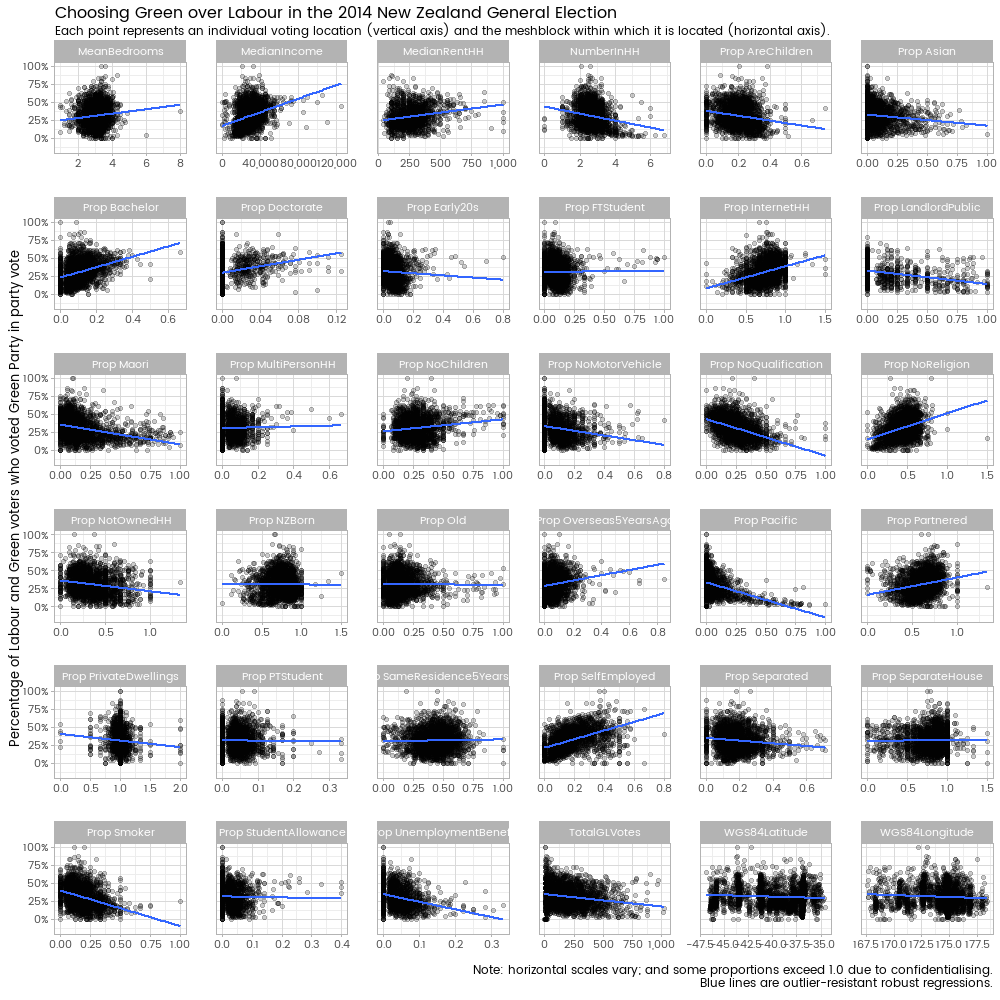
Full descriptions of the variables are in the helpfile for the Meshblocks2013 object in the nzelect package. People without access to that can still read the source code of the helpfile which hopefully will make sense. Time and space constraints put me off creating a big table here in this blog post.
The blue lines show outlier-resistant robust linear regressions on one explanatory variable at a time, but the non-robust versions are almost identical. All code has been relegated to the bottom of the post. When the nzelect package has a more complete set of census data, including more variables and area unit, electorate and territorial authority variables, I’ll do a future post that focuses more on the code to join these things together.
Two variables that are in the nzelect package have been excluded. These are PropEuropean, the proportion of meshblock population of European ethnicity; and PropOwnResidence, the proportion of individuals that own their own residence. I excluded these early as part of my modelling strategy because they are highly collinear with the other set of candidate explanatory variables - variance inflation factors over 10. What this means in practice is that once you know the proportions of Maori, Asian and Pacific ethnicity in a meshblock there’s not much to learn from the proportion of people of European ethnicity. And once you know the proportion of households that are owned, there’s not much information contained in knowing the proportion of individuals who own their residence.
Spatial elements
Note that I’ve left in two variables for the latitude and longitude, which (probably as expected) don’t have any obvious relationship to the proportion of Green v Labour voters. This is so when I get into statistical modelling, I can take into account expected spatial auto-correlation. Simply put, that means that the results from two voting places that are close together shouldn’t be treated as completely fresh independent information, but given somewhat less importance because of their co-location. This is just a nuisance aspect of the model with regard to today’s question so I don’t report on the results; but in the modelling I do later I make sure I have a spatial spline lurking in the background to suck up any spatial effects, leaving the estimates of the impact of other explanatory variables safer.
Imputation
For confidentialisation, meshblock census results are subject to random rounding (which is why some of the proportions exceed 1 - the numerator has been rounded one way, and the denominator another) and to outright cell suppression. For today’s purposes, the cell suppression is more of a problem. As I’ve potentially got lots of explanatory variables in my model, many meshblocks are missing at least one variable due to the confidentialisation. If I excluded each voting place whose meshblock was missing data, I’d be throwing out 61% of the data.
This is enough of a problem that I’d consider going up a level and using area units (larger shapes than meshblocks) instead, although many area units have multiple voting locations in them so we would lose a fair bit of granularity in doing so. However, the nzelect data doesn’t yet include its area unit slice and I’m short of time, so I opt for imputation instead.
I use multiple imputation, which means that you create statistical models to predict each missing value based on the values that you do have, and do this multiple times for each missing value, including the random element of the model and hence getting a different imputed value each time. Then when you fit your final model of actual interest you fit it to each one of your datasets with missing value imputations (in this example I have 20 full sets of the data) and you base your calculations of standard errors, confidence intervals, etc. on the randomness that comes from the imputation process as well as the usual modelling uncertainty. It’s not a fool-proof method - nothing is in the face of missing data - but it’s a good one and it does the job in this case (how do I know? I tried other methods, including deleting all rows, and got similar results).
Modelling
When it comes to the actual modelling I use a generalised additive model with a binomial family response. The ‘additive’ bit comes from a flexible two dimensional spline which is just there to deal with the nuisance of the spatial autocorrelation. The binomial family response is appropriate for the data which uses proportions. Here’s the end results showing which variables are good for predicting the proportion of Green / Labour votes that are for the Green Party:

Interpretation
So, just to be really clear, here are the factors in the surrounding meshblock that seem lead to a voting place returning a high proportion of Green/Labour voters voting Green:
- Higher proportion of individuals are self employed
- Higher proportion of individuals have a Bachelor degree
- Higher proportion of individuals have no religion
- Higher proportion of individuals were overseas 5 years ago
- Higher proportion of households don’t own their residence
And here are the factors that are associated with a high proportion of Green/Labour voters voting Labour:
- High proportion of individuals state they are of Pacific, Asian or Maori ethnicity
- High proportion of individuals have no qualifications
- High proportion of individuals were born in New Zealand
- High proportion of individuals have partner or are separated
- Higher individual median income
- Higher proportion of individuals are aged 20 to 24
There’s no discernable impact from the median household rent, best proxy in the particular data available for household prices. So on the data available, the general demographics argument wins over the housing prices one.
The surprising one here was the negative coefficient in front of median income. This differs from the simple two variable relationship seen in the first graphic in this post; what we’re seeing with the more sophisticated modelling is evidence that the apparent relationship between income and higher proportions of Green voters over Labour is a proxy for other demographic factors (like education, ethnicity and employment), and when those factors are controlled for the relationship between income and choosing Green over Labour is negative.
Care needs to be taken in leaping from this analysis to conclusions about individual behaviour, which would form the ecological fallacy. For example, while areas with higher incomes seem more inclined to choose Labour over Green after controlling for other factors, it’s at least possible that it’s being surrounded by higher income people that has the effect, rather than being higher income oneself; and similarly with any other observed effect. But with caution and caveats you can at least form some tentative conclusions about individuals; only individual level data could resolve that, and the New Zealand Election Study (which would provide that) isn’t yet available for download.
Final warnings
One thing we don’t do at this point is knock out all those “non significant” variables like proportion of people on unemployment benefit, proportion who are full time students, etc and refit the model. This leads to all the standard errors being biased downwards, the effect sizes being biased upwards, test statistics not having the claimed distributions, confidence intervals being too small, and in fact pretty much any inference after that point is invalid. This doesn’t stop that kind of stepwise model building from being common practice, but don’t let me catch you doing it in a context where inference about effect sizes and “which variables have how much explanatory power” are important (sometimes for predictive models that stepwise approach is more justifiable, if done carefully).
This analysis is incomplete because the nzelect project is incomplete. Most glaringly, two whole sets of individual level census variables have been excluded simply because I didn’t get round to including them in the original data package. This doesn’t invalidate the findings but it does add extra cautions and caveats. I’ll fix that eventually but it might be a few months away.
OK, that’s enough to go along with. Thanks for reading. Here’s the code that did that analysis:
#---------load up functionality and fonts------------
devtools::install_github("ellisp/nzelect/pkg")
devtools::install_github("hadley/ggplot2") # latest version needed for subtitles and captions

library(MASS) # for rlm().  Load before dplyr to avoid "select" conflicts
library(mice) # for multiple imputation
library(dplyr)
library(tidyr)
library(ggplot2)
library(scales)
library(showtext)
library(car)      # for vif()
library(ggthemes) # for theme_tufte
library(mgcv)     # for a version of gam with vcov() method
font.add.google("Poppins", "myfont")
showtext.auto()
theme_set(theme_light(10, base_family = "myfont"))

# load in the data
library(nzelect)

#-----------general data prep------------
# Some voting places don't have a match to mesthblock and hence aren't any
# good for our purposes.  Note - Chatham Islands *should* be a match, but that
# an issue to fix in the nzelect package which we'll ignore for now
bad_vps <- c(
   "Chatham Islands Council Building, 9 Tuku Road, Waitangi",
   "Ordinary Votes BEFORE polling day",
   "Overseas Special Votes including Defence Force",
   "Special Votes BEFORE polling day",
   "Special Votes On polling day",
   "Votes Allowed for Party Only",
   "Voting places where less than 6 votes were taken")

GE2014a <- GE2014 %>%
   filter(!VotingPlace %in% bad_vps)


#------------Greens / (Greens + Labour)--------------
# make a dataset with the response variable we want (Greens / (Greens + Labour))
# and merged with the VotingPlace locations and the relevant meshblock data
greens <- GE2014a %>%
   filter(VotingType == "Party" &
             Party %in% c("Green Party", "Labour Party")) %>%
   group_by(VotingPlace) %>%
   summarise(PropGreens = sum(Votes[Party == "Green Party"]) / sum(Votes),
             TotalGLVotes = sum(Votes)) %>%
   ungroup() %>%
   left_join(Locations2014, by = "VotingPlace") %>%
   left_join(Meshblocks2013[ , 1:55], by = c("MB2014" = "MB")) %>%
   select(PropGreens, TotalGLVotes, WGS84Latitude, WGS84Longitude,
          MeanBedrooms2013:PropStudentAllowance2013)

# Tidy up names of variables.  All the census data is from 2013 so we don't
# need to say so in each variable:
names(greens) <- gsub("2013", "", names(greens))


# Identify and address collinearity in the explanatory variables
mod1 <- lm(PropGreens ~ . , data = greens)
sort(vif(mod1) )
# PropEuropean is 17 - can be predicted from maori, Pacific Asian.
# PropOwnResidence is 11 - can be predicted from PropNotOwnedHH
# so let's take those two un-productive variables out
greens <- greens[ , !names(greens) %in% c("PropEuropean", "PropOwnResidence")]


# Image of scatter plots of explanatory variables v response variable
png("../img/0038-green-labour.png", 1000, 1000, res = 100)
greens %>%
   gather(Variable, Value, -PropGreens) %>%
   mutate(Variable = gsub("2013", "", Variable),
          Variable = gsub("Prop", "Prop ", Variable)) %>%
   ggplot(aes(x = Value, y = PropGreens)) +
   facet_wrap(~Variable, scales = "free_x", ncol = 6) +
   geom_point(alpha = 0.2) +
   geom_smooth(method = "rlm", se = FALSE) +
   scale_y_continuous("Percentage of Labour and Green voters who voted Green Party in party vote",
                      label = percent) +
   scale_x_continuous("", label = comma) +
   labs(caption = "Note: horizontal scales vary; and some proportions exceed 1.0 due to confidentialising.\nBlue lines are outlier-resistant robust regressions.") +
   ggtitle("Choosing between Labour and Green in the 2014 New Zealand General Election",
      subtitle = "Each point represents an individual voting location (vertical axis) and the meshblock within which it is located (horizontal axis).") +    theme(panel.margin = unit(1.5, "lines"))
dev.off()


# More data munging prior to model fitting

# only 39% of cases are complete, due to lots of confidentialisation:
sum(complete.cases(greens)) / nrow(greens)
# so to avoid chucking out half the data we will need to impute.  Best way
# is multiple imputation, which gives

# to make it easier to compare the ultimate coefficients, we're going to
# scale the explanatory variables.  Easiest to do this before imputationL
greens_scaled <- greens
greens_scaled[ , -(1:2)] <- scale(greens_scaled[ , -(1:2)] )

# Now we do the multiple imputation.
# Note that we ignore PropGreens for imputation purposes - don't want to impute
# the Xs based on the Y!  First we define the default predictor matrix:
predMat <- 1 - diag(1, ncol(greens_scaled))
# Each row corresponds to a target variable, columns to the variables to use in
# imputing them.  We say nothing should use PropGreens (first column).  Everything
# else is ok to use, including latitude and longitude and the total green and labour
# votes:
predMat[ , 1] <- 0
greens_mi <- mice(greens_scaled, m = 20, predictorMatrix = predMat)

# what are all the variable names?:
paste(names(greens_scaled)[-1], collapse = " + ")

# fit models to each of the imputed datasets:
mod2 <- with(greens_mi,
             gam(PropGreens ~ MeanBedrooms + PropPrivateDwellings +
                   PropSeparateHouse + NumberInHH + PropMultiPersonHH +
                   PropInternetHH + PropNotOwnedHH + MedianRentHH +
                   PropLandlordPublic + PropNoMotorVehicle + PropOld +
                   PropEarly20s + PropAreChildren + PropSameResidence5YearsAgo +
                   PropOverseas5YearsAgo + PropNZBorn + PropMaori +
                   PropPacific + PropAsian + PropNoReligion + PropSmoker +
                   PropSeparated + PropPartnered + PropNoChildren +
                   PropNoQualification + PropBachelor + PropDoctorate +
                   PropFTStudent + PropPTStudent + MedianIncome +
                   PropSelfEmployed + PropUnemploymentBenefit +
                   PropStudentAllowance +
                    s(WGS84Latitude) + s(WGS84Longitude) +
                    s(WGS84Latitude * WGS84Longitude),
                family = binomial, weights = TotalGLVotes)
)


# extract all the estimates of coefficients, except the uninteresting intercept:
coefs <- summary(pool(mod2))[-1, ]
vars <- rownames(coefs)
coefs <- as.data.frame(coefs) %>%
   mutate(variable = vars) %>%
   arrange(est) %>%
   mutate(variable = gsub("Prop", "", variable)) %>%
   mutate(variable = factor(variable, levels = variable)) %>%
   # drop all the uninteresting estimates associated with the spatial splines:
   filter(!grepl("WGS84", variable))

# make names referrable:
names(coefs) <- gsub(" ", "_", names(coefs), fixed = TRUE)

# define plot of results:
p2 <- ggplot(coefs, aes(x = variable, ymin = lo_95, ymax = hi_95, y = est)) +
   geom_hline(yintercept = 0, colour = "lightblue") +
   geom_linerange(colour = "grey20") +
   geom_text(aes(label = variable), size = 3, family = "myfont", vjust = 0, nudge_x = 0.15) +
   coord_flip() +
   labs(y = "\nHorizontal lines show 95% confidence interval of scaled impact on
proportion that voted Green out of Green and Labour voters.
The numbers show coefficients from a logistic regression and
should be taken as indicative, not strictly interpretable.\n",
        x = "",
        caption = "Source: http://ellisp.github.io") +
   ggtitle("Census characteristics of voting places that party-voted Green over Labour",
      subtitle = "New Zealand General Election 2014") +
   theme_tufte(base_family = "myfont") +
   theme(axis.text.y = element_blank(),
         axis.ticks.y = element_blank()) +
   annotate("text", y = -0.2, x = 6, label = "More likely to\nvote Labour",
            colour = "red", family = "myfont") +
   annotate("text", y = 0.18, x = 31, label = "More likely to\nvote Green",
            colour = "darkgreen", family = "myfont")

print(p2)