So a critical discussion of Sankey plots floated across my feed on Bluesky recently, and one reply included an ugly example and the comment “Anybody who thought that this illustration enhanced clarity lives in an alternative reality”. The actual chart I’ve included at the bottom of this post. I agree it’s pretty unhelpful, but I thought I saw potential, and said so. This blog is me seeing if in fact something can be done with it.
The post that started the discussion was Emily Moin saying “Sankey diagrams are just as bad as pie charts, and also worse because conventional wisdom has not rejected them yet so I still have to look at them”. As it happens, I think that even pie charts have their (very limited) place so long as they are carefuly chosen (not when too many categories, for example) and properly polished for the audience. So I guess I am being consistent in thinking that Sankey charts can also be useful.
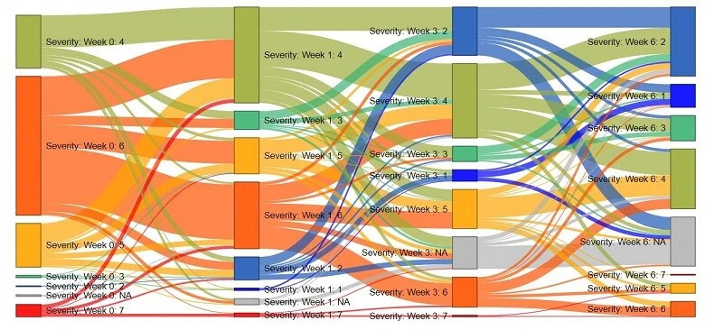
Here’s what I think is wrong with the original graphic (which is reproduced later in this post), which I think is tracking the progression of patients experiencing symptoms of varying severity over a period of six weeks:
- The labels clutter the image and have a lot of redundant information repeated multiple times (“Severity Week…”)
- The weeks and severity are both measured in numbers and presented together in the labels, making a significant cognitive load to parse the labels (“Severity Week 0: 3” takes some effort to work out the severity is 3 and the week is 0, which is exactly the sort of thing you want to intuit directly from position or colour in a plot rather than have to read it)
- The colours aren’t colour-blind friendly.
- Although the colours are mapped appropriately to the severity scale (blue for low severity, green to mid and red for high) there’s no legend to draw this to the reader’s attention, and because of the ordering of ribbons on the page (see next point) this sequencing of colours is never obvious to the reader.
- The nodes representing severity in a given week aren’t in any fixed order on the page, and change from week to week. They seem to have been chosen more to get the severity levels with more patients towards the centre of the chart. This stops the reader getting any easy reading of severity (which could have been mapped to vertical position in the plotting area) and adds to the cluttered and complex feel of the plot - for example by having the blue ribbon for severity 2 jumping from near the bottom of the plot in weeks 0 and 1 to the top in weeks 3 and 6.
You’ll need to go down a bit in the post to see that original graphic; you’ll see that the combined effect of these problems is indeed one of complexity and clutter. I think the last point - the severity nodes swapping places vertically - is the most important.
I had a go at improving this and came up with a couple of alternatives, using David Sjoberg’s ggsankey R package. Here’s a Sankey plot version:
… and here’s an alluvial plot version. Alluvial plots are similar to Sankey plots but have no spaces between the nodes, which means in this case you can read the nodes vertically at each week similarly to a stacked bar chart:
Here’s the original graphic for comparison:
I’m pretty confident that either the Sankey or alluvial plot are definite improvements and give a better sense of the average severity in each week, and the overall trend (which is more blue, low severity cases). While still giving a sense of people moving in multiple directions (sometimes upwards) from each severity-week combination. So I think I’ve addressed the main points here:
- Decluttered the labels by having axis labels for “Week zero”, “Week one”, etc; meaning we don’t need to repeat this in each node. And the node label is now just the single number of the severity.
- Avoided the cognitive load of week and severity both being numerals, partly by the simplified labels above and partly by spelling out weeks in English words (one, three, etc) rather than numerals.
- Chosen a more colour-blind friendly palette based on the Brewer Red-Yellow-Blue scheme rather than Red-Green-Blue
- I still don’t have a legend, but I think it is now much clearer to the reader that red is high severity and blue is low, because of the vertical sequencing of the nodes…
- … which is the main fix here - I’ve strictly ordered the 1,2,3,4,5,6,7 severity nodes vertically so they never swap positions. This means less crossing-of-the-beams and hence less feel of complexity in the plot. Most importantly, it gives the eye an easy way to judge the proportion of people in each severity level by vertical position and size on the page.
I’ve left all the code at the end because most of it was about me trying to put together by hand a dataset that resembles that in the original flow chart. Then I had to calibrate it in R to fix the problems in my hand-made version. This included problems like the number of people changing from week to week, and the number of people entering a particular severity state in one week not matching the number exiting it. Once that stuff is dealt with, drawing the actual plot is a relatively simple ggplot2 and ggsankey chunk of code.
library(tidyverse)
library(janitor)
library(glue)
library(RColorBrewer)
remotes::install_github("davidsjoberg/ggsankey")
library(ggsankey) # one fairly straightforward approach to sankey charts / flow diagrams

# read in some data. This was very crudely hand-entered with some
# rough visual judgements based from a chart that I don't know the
# origin of I saw on the internet. So treat as made-up example data:
d <- read_csv("https://raw.githubusercontent.com/ellisp/blog-source/refs/heads/master/data/complicated-sankey-data.csv",
              col_types = "ccccd",
              # we want the NAs in the original to be characters, not actual NA:
              na = "missing") |>
  clean_names()

#------------tidying up data---------------
# we have some adjustments to deal with because of having made up data

# An extra bunch of rows of data that are needed by the Sankey function to
# to make the week 6 nodes show up:
extras <- d |>
  filter(week_to == "6") |>
  mutate(
    week_from = "6",
    week_to = NA,
    severity_from = severity_to)

#' Convenience relabelling function for turning week numbers into a factor:
weekf <- function(x){
  x <-  case_when(
    x == 0 ~ "Week zero",
    x == 1 ~ "Week one",
    x == 3 ~ "Week three",
    x == 6 ~ "Week six"
  )
  x <- factor(x, levels = c("Week zero","Week one","Week three", "Week six"))
}

# going to start by treating all flow widths as proportions
total_people <- 1

# add in the extra data rows to show the final week of nodes,
# and relabel the weeks:
d2 <- d |>
  rbind(extras)  |>
  mutate(week_from =  weekf(week_from),
         week_to = weekf(week_to))

# there should be the same total number of people each week,
# and the same number of people leaving each "node" (a severity-week
# combination) as arrived at it on the flow from the last week.
# we have a little iterative process to clean this up. If we had
# real data, none of this would be necessary; this is basically
# because I made up data with some rough visual judgements:
for(i in 1:5){
  # scale the data so the population stays the same week by week
  # (adds up to total_people, which is 1, so are proportions)
  d2 <- d2 |>
    group_by(week_from) |>
    mutate(value = value / sum(value) * total_people) |>
    group_by(week_to) |>
    mutate(value = value / sum(value) * total_people) |>
    ungroup()

  # how many people arrived at each node (week-severity combination)?
  tot_arrived <- d2 |>
    group_by(week_from, severity_from) |>
    mutate(arrived_sev_from = sum(value)) |>
    group_by(week_to, severity_to) |>
    mutate(arrived_sev_to = sum(value)) |>
    ungroup() |>
    distinct(week_to, severity_to, arrived_sev_to)

  # scale the data leaving the node to match what came in:
  d2 <- d2 |>
    left_join(tot_arrived, by = c("week_from" = "week_to",
                                  "severity_from" = "severity_to")) |>
    group_by(week_from, severity_from) |>
    mutate(value = if_else(is.na(arrived_sev_to), value,
                                 value / sum(value) * unique(arrived_sev_to)) ) |>
    select(-arrived_sev_to) |>
    ungroup()
}

# manual check - these should all be  basically the same numbers
filter(tot_arrived, week_to == "Week one" & severity_to == 4)
filter(d2, week_to == "Week one" & severity_to == 4) |> summarise(sum(value))
filter(d2, week_from == "Week one" & severity_from == 4) |> summarise(sum(value))


#--------------draw plot-------------

# palette that is colourblined-ok and shows sequence. This
# actually wasn't too bad in the original, but it got lost
# in the vertical shuffling of all the severity nodes:
pal <-  c("grey", brewer.pal(7, "RdYlBu")[7:1])
names(pal) <- c("NA", 1:7)

# Draw the actual chart. First, the base of chart, common to both:
p0 <- d2 |>
  mutate(value = round(value * 1000)) |>
  uncount(weights = value) |>
  mutate(severity_from = factor(severity_from, levels = c("NA", 1:7)),
         severity_to = factor(severity_to, levels = c("NA", 1:7))) |>
  ggplot(aes(x = week_from,
             next_x = week_to,
             node = severity_from,
             next_node = severity_to,
             fill = severity_from,
             label = severity_from)) +
  # default has a lot of white space between y axis and the data
  # so reduce the expansion of x axis to reduce that
  scale_x_discrete(expand = c(0.05, 0)) +
  scale_fill_manual(values = pal) +
  labs(subtitle = "Chart is still cluttered, but decreasing severity over time is apparent.
To achieve this, vertical sequencing is mapped to severity, and repetitive labels have been moved into the axis guides.",
       x = "",
       caption = "Data has been hand-synthesised to be close to an original plot of unknown provenance.")

# Sankey plot:
p1 <- p0 +
  geom_sankey(alpha = 0.8) +
  geom_sankey_label() +
  theme_sankey(base_family = "Roboto") +
  theme(legend.position = "none",
        plot.title = element_text(family = "Sarala")) +
  labs(title = "Severity of an unknown disease shown in a Sankey chart")

# Alluvial plot:
p2 <- p0 +
  geom_alluvial(alpha = 0.8) +
  geom_alluvial_label() +
  theme_alluvial(base_family = "Roboto") +
  theme(legend.position = "none",
        plot.title = element_text(family = "Sarala")) +
  labs(title = "Severity of an unknown disease shown in an alluvial chart",
       y = "Number of people")

print(p1) # Sankey plot
print(p2) # alluvial plot