Linear model with time series random component

What do auto-correlated residuals do to your linear model?

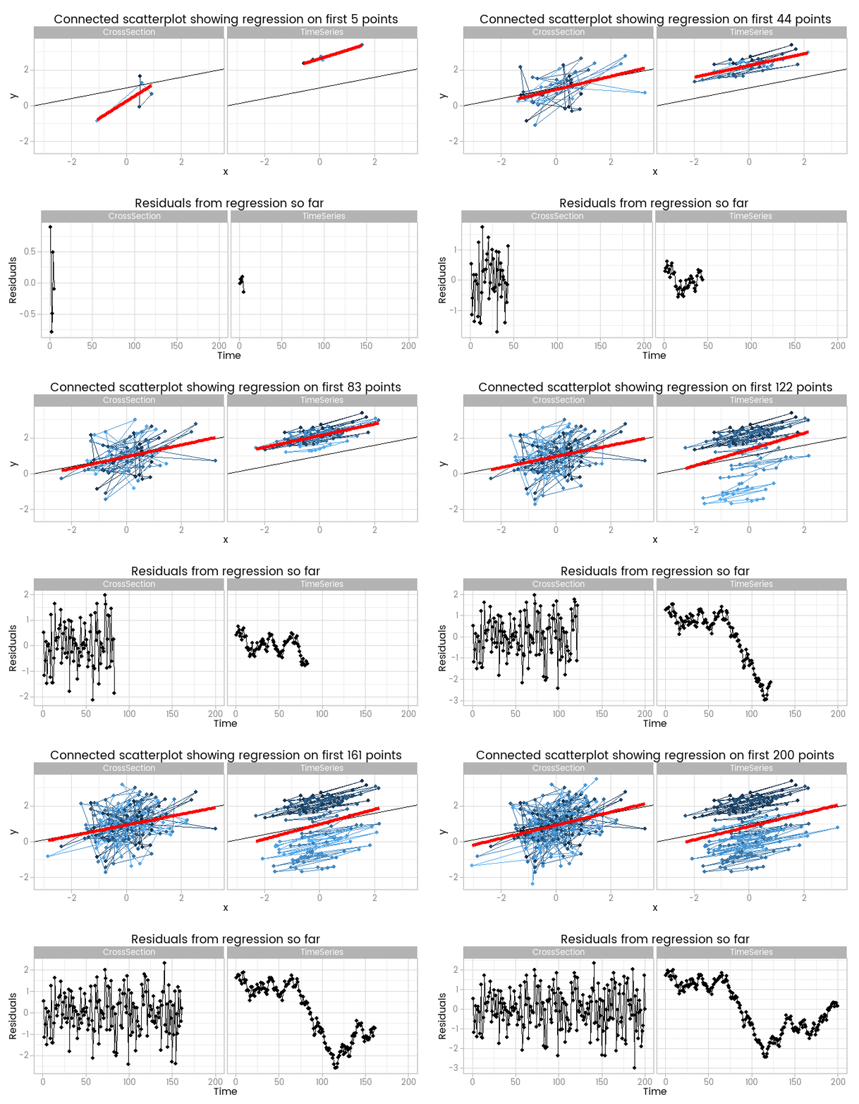
For training purposes I wanted to illustrate the dangers of ignoring time series characteristics of the random part of a classical linear regression, and I came up with this animation to do it:

I like this, because it shows how easy it is to fit something that looks to be a good fit but actually misses important parts of reality. The red lines show where the fitted model is, based on a small window of the data - from 5 to 200 points. The black line shows the true data generating process. From very early on the model fit to the simple cross-sectional has converged to pretty close to the black line. However, the model fit to the data with time series errors spends a long time greatly overestimating the value of one of the parameters in the model, and not until there are 120 observations has it converged to anywhere near the true process.

At the very least, it shows that you need many more - four times as many in this case, but unfortunately that’s not a magic number that will always work - observations from a time series to reliably estimate the structural part of a model. Even if we’d explicitly modelled the time series part of the data on the right of the animation, we’d still have that problem.

By including the residual plots below the scatter plots we get a nice picture of a warning sign in this basic (and should be fundamental and universal) diagnostic plot. In this particular case the pattern is obvious; when working with real data you should check with partial autocorrelation function plots too.

Simulating data

The animation illustrates the results of simulating and contrasting two fairly extreme cases:

• cross section data, generated exactly from a model of y = a + b.x + e, e ~ N(0, 1). This is the textbook case introduced in any basic statistics course;
• time series data, generated with exactly the same model except the error term, in addition to be normally distributed with mean of zero and standard deviation of 1, has a high autocorrelation.

I chose to make the intercept of my model (a in the above formulation) 1, and the slope (b) equal to 0.3. Here’s what the first 200 observations of the response variable looks like:

In fact, I’ve over-simplified things by leaving x in both datasets as independent and identically distributed white noise. In reality, if y has a time series random component, x probably will have too. But I wanted to illustrate how a single violation of our assumptions can lead to problems, rather than create a fully realistic case (which obviously would show up even more problems).

The data were generated as follows. To illustrate a point and make it a realistic test, I generate a much larger “population” time series, and the mean of zero and standard deviation of 1 applies only to that larger population. The first 200 points is all we see.

library(dplyr)
library(tidyr)
library(ggplot2)
library(gridExtra)
library(showtext)

#-------------set up-------------
# Fonts and themes:
font.add.google("Poppins", "myfont")
showtext.auto()
theme_set(theme_light(base_family = "myfont"))

# sample and population size:
n <- 200
popn <- n * 10


#----------simulate data---------
set.seed(123)

# Linear model with a time series random element, n * 10 in length:
df1 <- data.frame(x = rnorm(popn)) %>%
   mutate(y = 1 + 0.3 * x + scale(arima.sim(list(ar = 0.99), popn)),
          ind = 1:popn,
          type = "TimeSeries")
# cut back to just the first n points:
df1 <- df1[1:n, ]


# Same linear model, with i.i.d. white noise random element:
df2 <- data.frame(x = rnorm(n)) %>%
   mutate(y = 1 + 0.3 * x + rnorm(n),
          ind = 1:n,
          type = "CrossSection")

# draw the time series response:
p0 <- df1 %>%
   ggplot(aes(x = ind, y = y)) +
   geom_line() +
   labs(x = "Time") +
   ggtitle("Simulated response variable from linear model\nwith time series random element")
   

Creating the animation is straightforward graphics. I make use of ggplot2’s faceting feature to cut down on some code, drawing the top two connected scatterplot images with one chunk and the bottom two residuals with another. Each frame is saved as an individual PNG image, and ImageMagick ties it all together into an animated GIF as easily as usual.

df_both <- rbind(df1, df2)


for(i in 5:n){

   # I name the images i + 1000 so alphabetical order is also numeric
   png(paste0(i + 1000, ".png"), 700, 600, res = 100)
   
   df1_tmp <- df1[1:i, ]
   df2_tmp <- df2[1:i, ]
   
   residuals1 <- data.frame(res = residuals(lm(y ~ x, data = df1_tmp)), 
                            ind = 1:i, 
                            type = "TimeSeries")
   residuals2 <- data.frame(res = residuals(lm(y ~ x, data = df2_tmp)), 
                            ind = 1:i, 
                            type = "CrossSection")
   
   # connected scatter plots:
   p1 <- ggplot(df_both[c(1:i, (n + 1) : (n + i)), ], aes(x, y, colour = ind)) +
      facet_wrap(~type, ncol = 2) +
      geom_path() +
      geom_point() +
      geom_abline(intercept = 1, slope = 0.3) +
      geom_smooth(method = "lm", se = FALSE, size = 2, colour = "red") +
      theme(legend.position = "none") +
      xlim(range(df_both$x)) +
      ylim(range(df_both$y)) +
      ggtitle(paste("Connected scatterplot showing regression on first", i, "points"))
      
   
   # Residuals plots    
   p2 <- residuals1 %>%
      rbind(residuals2) %>%
      mutate(type = factor(type, levels = c("CrossSection", "TimeSeries"))) %>%
      ggplot(aes(x = ind, y = res)) +
      scale_x_continuous(limits = c(0, n)) +
      facet_wrap(~type) +
      geom_line() +
      geom_point() +
      ggtitle("Residuals from regression so far") +
      labs(x = "Time", y = "Residuals")
   
   grid.arrange(p1, p2)
   
   dev.off()
   
}

# combine them into an animated GIF
system('"C:\\Program Files\\ImageMagick-6.9.1-Q16\\convert" -loop 0 -delay 10 *.png "timeseries.gif"')