Motivation
For a variety of reasons I wanted a Linux server in the cloud with data science software on it. In no particular order:
- so I could access a reliable setup from anywhere with a web browser, including on networks without the software I need (which happens a lot in corporate/government environments)
- so I could do round-the-clock data gathering when necessary
- to run my pet HappyRrobot twitterbot, having retired the old physical linux box it used to be hosted from
- to make sure I stay familiar with what’s needed to set up such a system from scratch.
I couldn’t tell you which of these are the more important.
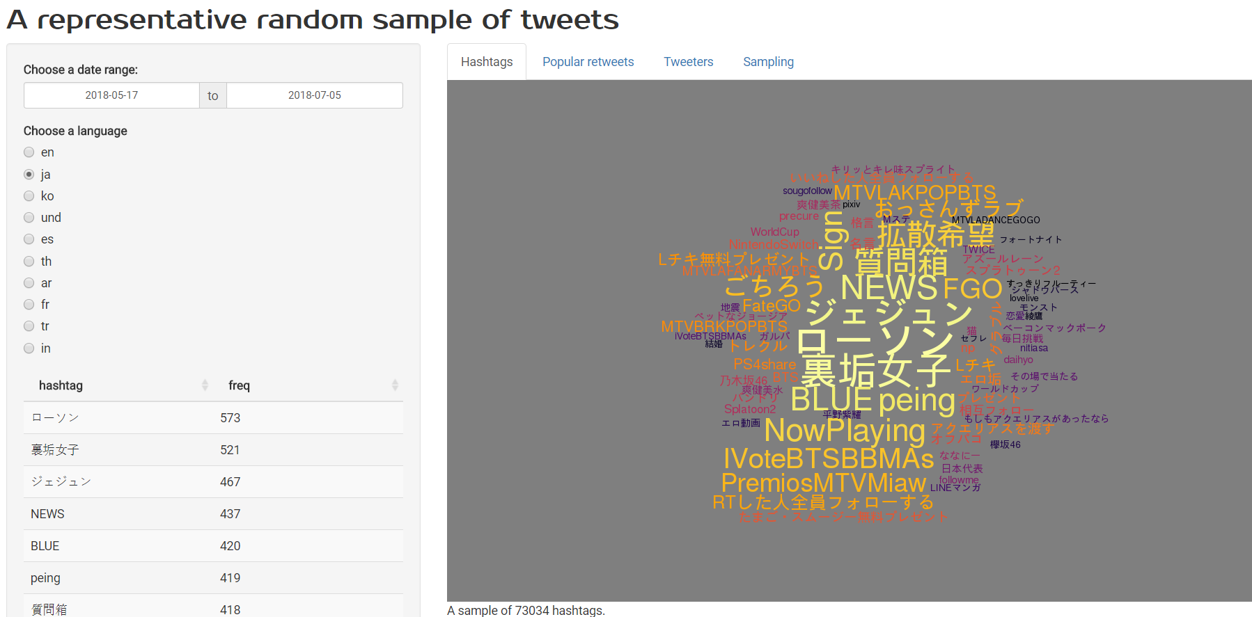
In this blog post I’ll be noting down the steps necessary for setting up this server, and illustrating purpose 2 with a Shiny app, hosted on the server and drawing data from a database on the server, which is collecting a round-the-clock random sample of Twitter. The end result looks like this (click on the image to go to the actual working app):
If you’re interested in Twitter data but not in setting up a Linux server with R, Shiny and PostgreSQL on it you can skip straight to where I talk about getting the data in and analysing it.
Setting up a server for data and stats
I chose Amazon Web Services Elastic Cloud to host the server. I used the Elastic IP service (fairly cheap) to allocate a permanent IP address to the instance.
I was keen on using Red Hat or similar flavoured Linux, because of purpose #4 noted above; I already knew a bit about Ubuntu and wanted to expand my knowledge sphere, and Red Hat is the flavour that seems to pop up on corporate and government servers. In the end I opted for CentOS, which is “a Linux distribution that provides a free, enterprise-class, community-supported computing platform functionally compatible with its upstream source, Red Hat Enterprise Linux (RHEL)”. In fact, installing R is a bit easier on CentOS that it was on my Red Hat experiments.
I want the following on this machine:
- R, RStudio Server and Python 3 for analysis and for data munging
- PostgreSQL for storing data and supporting analysis
- Shiny Server for dissemination
- A webserver (I chose Nginx) to support RStudio Server and Shiny Server through reverse proxy so I can access them on regular web browser ports rather than ports 8787 and 3838, which will often not be available from a corporate network
- all the other utilities and extras to support all this, such as curl, mail and fonts
This was non-trivial, which is one of the reasons why I’m blogging about it! There are lots of fishhooks and little things to sort through and while there are some excellent blog posts and tutorials out there to help do it, none of them covered quite the end-to-end setup I needed. One of my outputs from the process was a set of notes - not quite a single run-and-forget configuration script as you’d want in a professional setup, but fairly easy to use - that makes it easy to do similar in the future.
R and a few basics
Here’s where I started, once having started up the server (plenty of tutorials on how to do that provided by Amazon themselves and others). I start by installing R, including the epel “Extra Packages for Enterprise Linux” that are needed beforehand.
# we'll want mail later
sudo yum install -y mailx

#-----------------R and its dependencies------------------------
#install R.  We need epel first
sudo yum update -y
sudo yum install –y https://dl.fedoraproject.org/pub/epel/epel-release-latest-7.noarch.rpm
sudo yum install -y texlive
sudo yum install -y texinfo

# clean up
rm *.rpm

sudo yum install -y R

# and version control of course
sudo yum install -y git
Database
Next thing was to install PostgreSQL. I found it useful to install this before I started installing R packages, because some R packages that speak to PostgreSQL behave differently on installation depending on whether PostgreSQL is found on the machine or not
#=====================postgresql=======================
# install postgresql.  Good to do this before we start installing R packages
sudo yum install -y postgresql-server postgresql-contrib postgresql-devel

sudo postgresql-setup initdb

# stop to give postgres account a password for the operating system
sudo passwd postgres

# start the postgresql service
sudo systemctl start postgresql

# I think this next line means the database service restarts when the machine is rebooted
sudo systemctl enable postgresql
Extending R via packages and their dependencies
I find installing all the R packages I regularly use a harder job in Linux than Windows. I’m sorry, but I do. In particular, Windows installations of packages like gdal seems to look after upstream dependencies seamlessly and quietly. Not so on Linux. Here’s what I needed to do at the command line to get all the R packages I wanted installed.
#======================miscellaneous dependencies needed by R packages===============
# iBest to do this on a large instance, even if you only start it as big
# during the install.  8GB seems a minimum

#----------------tidyverse and Cairo---------
# First, some dependencies that rvest, devtools, Cairo need:
sudo yum install -y libcurl-devel libxml2-devel openssl-devel
sudo yum install -y cairo-devel  libXt-devel  udunits2-devel gdal-devel poppler-cpp-devel


#------------The gdal epic---------------------
# needed for spatial stuff and in particular sf which needs version > 2 (currently 2.2).
# This should work according to the sf github page (excluding udunits2 which we look after later):
sudo yum install -y gdal-devel proj-devel proj-epsg proj-nad geos-devel
# but that installs the wrong version of gdal!  We have to install it by hand.
# see https://gis.stackexchange.com/questions/263495/how-to-install-gdal-on-centos-7-4


# adapted from https://gist.github.com/simondobner/f859b2db15ad65090c3c316d3c224f45
wget http://download.osgeo.org/gdal/2.2.4/gdal-2.2.4.tar.gz
tar zxvf gdal-2.2.4.tar.gz
cd gdal-2.2.4/
./configure --prefix=/usr/ --with-sfcgal=no
make -j4
sudo make install

# should have a test here to only do the next two things if installed correctly!
rm *.tar.gz
rm gdal-2.2.4 -r

#======================R packages=====================
# Now we can install R packages that need all the above system dependencies first.
#
# udunits2 needs special configuration when installing in R so let's do that first and get it out of the way
sudo R -e "install.packages('udunits2',configure.args='--with-udunits2-include=/usr/include/udunits2', repos='http://cran.rstudio.com/')"

# these are a bunch of packages that are heavily used and that I want installed up front and available
# for all users (hence installing them as super user)
sudo R -e "install.packages(c('Rcpp', 'rlang', 'bindrcpp', 'dplyr', 'digest', 'htmltools', 'tidyverse',
'shiny', 'leaflet', 'sf', 'scales', 'Cairo', 'forecast', 'forcats', 'h2o', 'seasonal', 'data.table',
'extrafont','survey', 'forecastHybrid', 'ggseas', 'treemap', 'glmnet', 'ranger', 'RPostgres', 'igraph',
'ggraph', 'nzelect', 'tm', 'wordcloud', 'praise', 'showtext', 'ngram', 'pdftools', 'rtweet', 'GGally',
'ggExtra', 'lettercase', 'xgboost'), repos='http://cran.rstudio.com/')"

# fonts
sudo yum install dejavu-sans-fonts
sudo yum install -y google-droid-*-fonts
sudo yum install -y gnu-free-*-fonts
sudo R -e "extrafont::font_import(prompt = FALSE)"
I did all of this with my server set up as a “large” instance with 8GB of RAM. This particularly makes a difference when installing Rcpp. After all the initial is setup you can stop the instance, downsize it something cheaper, and restart it.
Note that I am using sudo to install R packages so they are available to all users (which will include the shiny user down the track), not just to me. I wanted everyone using this server to have the same set of packages available; obviously whether this is desirable or not depends on the purpose of the setup.
Server-related stuff
Next I want to get RStudio Server and Shiny Server working, and accessible via a web browser that just talks to standard port 80. There is a step here where the Nginx configuration file gets edited by hand; the links to RStudio support for RStudio Server and for Shiny Server contain instructions on what needs to go where.
Also note that the actual versions of RStudio Server and of Shiny Server below are date-specific (because they are installed via local install), and probably the links are already out of date.
#-------------webby stuff------------
# install a web server so we can deliver things through it via reverse proxy
# see  https://support.rstudio.com/hc/en-us/articles/200552326-Running-RStudio-Server-with-a-Proxy
# and https://support.rstudio.com/hc/en-us/articles/213733868-Running-Shiny-Server-with-a-Proxy
sudo yum install -y nginx

#install RStudio-Server (2018-04-23)
wget https://download2.rstudio.org/rstudio-server-rhel-1.1.447-x86_64.rpm
sudo yum localinstall -y --nogpgcheck rstudio-server-rhel-1.1.447-x86_64.rpm

#install shiny and shiny-server (2018-04-23)

wget https://download3.rstudio.org/centos6.3/x86_64/shiny-server-1.5.7.907-rh6-x86_64.rpm
sudo yum localinstall -y --nogpgcheck shiny-server-1.5.7.907-rh6-x86_64.rpm
rm *.rpm

# now go make the necessary edits to /etc/nginx/nginx.conf
# note that the additions are made in two different bits of that file, you don't just past the whole
# lot in.

sudo nano /etc/nginx/nginx.conf

sudo systemctl restart nginx
# go to yr.ip.number/shiny/ and yr.ip.number/rstudio/ to check all working

# add some more users if wanted at this point
# sudo useradd ellisp
# sudo passwd ellisp

# not sure if all these are needed:
sudo systemctl enable nginx
sudo systemctl enable rstudio-server
sudo systemctl enable shiny-server

# set the ownership of the directory we're going to keep apps in so the `shiny`
# user can access it
sudo chown -R shiny:shiny /srv/shiny-server
Python
Centos currently comes with Python 2.7, but I wanted to be using Python 3. My Python skills are halting at best but I want them to be as future-proofed as possible. Anaconda seems a relatively straightforward way to manage Python.
#---------------Anaconda / python----------------
# go to https://repo.continuum.io/archive/ or https://www.anaconda.com/download/#linux to see the latest version
# Anaconda3 is with python 3.X, Anaconda2 is wit python 2.7.  Note
# that python 2.7 is part of the Centos linux dsitribution and shouldn't be
# overwritten ie python xxx.py  should run python 2.7.  But doing the process below does this;
# watch out for if this causes problems later...
#
wget https://repo.continuum.io/archive/Anaconda3-5.1.0-Linux-x86_64.sh
sudo bash Anaconda3-5.1.0-Linux-x86_64.sh
# agree to the license, and specify /opt/anaconda3 as location when asked

# we want to give all users anaconda on their path, so I snitched this from:
# https://www.vultr.com/docs/how-to-install-jupyter-notebook-on-a-vultr-centos-7-server-instance
sudo cp /etc/profile /etc/profile_backup
echo 'export PATH=/opt/anaconda3/bin:$PATH' | sudo tee -a /etc/profile
source /etc/profile
echo $PATH

sudo /opt/anaconda3/bin/conda conda install psycopg2

# as far as I can tell this makes python3.6 the default python, which is surely going to cause problems down
# the track...
Configuring PostgreSQL
I installed PostgreSQL and started its database service early in this process, but in the next step need to actually set up some database and users for use. The PostgreSQL security model is thorough and comprehensive but with lots of fishhooks. Here’s how I set it up for this particular (very simple) use case. First, I enter the psql environment as the postgres user (currently the only user with any access to the database server)
sudo -u postgres psqlNow we can set up the users we want to be accessing our databases; some databases for them to use; and schemas within those database. In this case, I set up two databases for now
survey_microdatatwitter
and three different users, in addition to postgres:
ellisp(ie me, in development mode)external_analyst(ie me or others, in read-only mode)shiny(the Shiny Server’s id on the server, needed so Shiny apps can access the database)
-- you are now in psql as user postgres.  Although default is to use unix's identification of you,
-- and you don't need a password to access the database from the local host, it's good to have a
-- password if you want to set up other connections later
\password postgres

CREATE DATABASE survey_microdata;
CREATE DATABASE twitter;

CREATE ROLE ellisp;
\password ellisp;
ALTER ROLE ellisp WITH LOGIN;

CREATE ROLE shiny;
-- no need for a password for shiny, it can only access the db from this machine

CREATE ROLE external_analyst;
\password external_analyst;

GRANT ALL PRIVILEGES ON DATABASE twitter TO ellisp;
GRANT ALL PRIVILEGES ON DATABASE survey_microdata TO ellisp;

\c survey_microdata;
CREATE SCHEMA nzivs;
CREATE SCHEMA nzis2011;
GRANT ALL PRIVILEGES ON SCHEMA nzivs TO ellisp;
GRANT ALL PRIVILEGES ON SCHEMA nzis2011 TO ellisp;
GRANT ALL PRIVILEGES ON ALL TABLES IN SCHEMA nzivs TO ellisp;
GRANT ALL PRIVILEGES ON ALL TABLES IN SCHEMA nzis2011 TO ellisp;

GRANT SELECT ON ALL TABLES IN SCHEMA nzis2011 to external_analyst;
GRANT SELECT ON ALL TABLES IN SCHEMA nzivs to external_analyst;

\c twitter
CREATE SCHEMA tweets;
GRANT ALL PRIVILEGES ON ALL TABLES IN SCHEMA public TO ellisp;
GRANT ALL PRIVILEGES ON ALL TABLES IN SCHEMA tweets TO ellisp;
GRANT SELECT ON ALL TABLES IN SCHEMA tweets TO shiny;
GRANT CONNECT ON DATABASE twitter TO shiny;
\q
We also need to tweak the configuration so the PostgreSQL database is accessible from the outside world (if that’s what we want, which I do).
# follow instructions at https://blog.bigbinary.com/2016/01/23/configure-postgresql-to-allow-remote-connection.html if
# you want to remotely access eg from DBeaver on your laptop.  Definitely need a password then
# first add in listen_addresses = 'localhost' just above the commented out version of #listen_addresses = 'localhost'
sudo nano /var/lib/pgsql/data/postgresql.conf

# now the client authentication file about how individuals can actually log on.
# Add the below two lines (not the # at beginning) to the bottom of the table.
# lets users log on via password form anywhere.  If this doesn't suit your
# risk profile, find something more constrictive...
# host    all             all              0.0.0.0/0                       md5
# host    all             all              ::/0                            md5
sudo nano /var/lib/pgsql/data/pg_hba.conf

sudo systemctl restart postgresql
A Twitter sample stream database
Collecting data
OK, that wasn’t so bad was it (or was it…). I now have my server running (I stopped it and restarted it as a smaller cheaper instance than the 8GB of RAM I used during that setup) and available to do Useful Stuff. Like collect Twitter data for analysis and dissemination in Shiny:
For a while, I’ve been mildly exercised by the problem of sampling from Twitter. See for example this earlier post where I was reduced to using a snowballing network method to find users, and searching for tweets with the letter “e” in them to get a sample of tweets. Both of these methods have obvious problems if you want to do inference about how people as a whole are using Twitter.
On the other hand, Twitter make available several sets of public Tweets that are fully representative:
- The free Sample Tweets API “returns a small random sample of all public Tweets.”
- The Decahose stream provides a 10% sample of all public Tweets
- The Firehose provides all public tweets
The latter two services are for paying customers only. My interest in Twitter is curiousity at most, so I’m only interested in the free sample, which is thought to be around 1% of the Firehose (exactly what proportion it is of the Firehose isn’t publicly known, and is a question of some inferential interest).
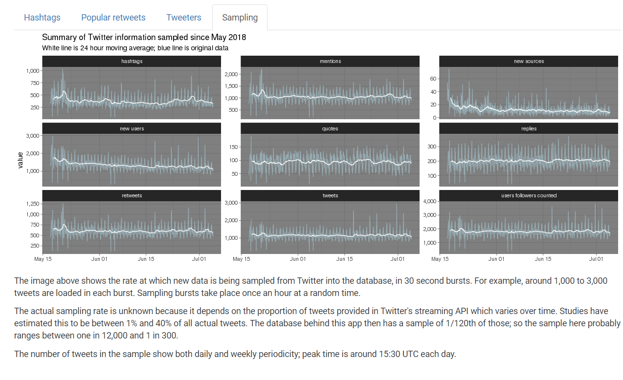
So I was interested in the sample stream, but I wanted to collect a sample over a period of time, not just from the day I was going to do some analysis. Even this 1% sample was more than I wanted to pay disk space to store if I were to collect over time, so I decided I would collect 30 seconds of sample streaming data every hour, at a random time within the hour to avoid problems associated with doing the sampling at the same time each day.
I designed a data model to capture the data I was most interested in while discarding attached video and images (this was about saving me disk space; I think serious Twitter analysis would have to do better than just collecting text). It looks like this:
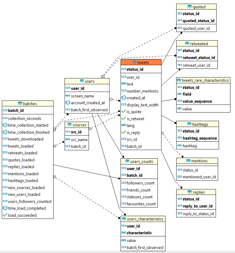
BTW that diagram (and much of the database development) was done with the excellent universal SQL editor and database admin tool, DBeaver. It works with different flavours of relational database and is awesome.
The code that creates and populates that database is available on GitHub:
- the SQL that builds the empty database.
- the R code that imports a 30 second window of the sample stream and uploads it to the
publicschema of thetwitterdatabase. All the heavy lifting is done by the awesome rtweet package. - the SQL that transforms and loads the data into the
twitter.tweetsschema. This does the work, for example, of matching users in the latest sample with previously observed users; making sure that re-tweeted users are in theuserstable even if we haven’t seen them directly tweet something themselves; and so on. - the shell script that is activated by a cron job 24 times a day and runs the above R and SQL.
This has now been running smoothly since 17 May 2018, apart from one day last week when I botched an R upgrade and it all went down for half a day before I noticed (lesson learned - run update.package(ask = FALSE, checkBuilt = TRUE) to ensure your R packages all keep working after the R internals change). So far the database is about 3GB in size, and I’m quite happy to let it grow quite a bit more than that.
What do we find out?
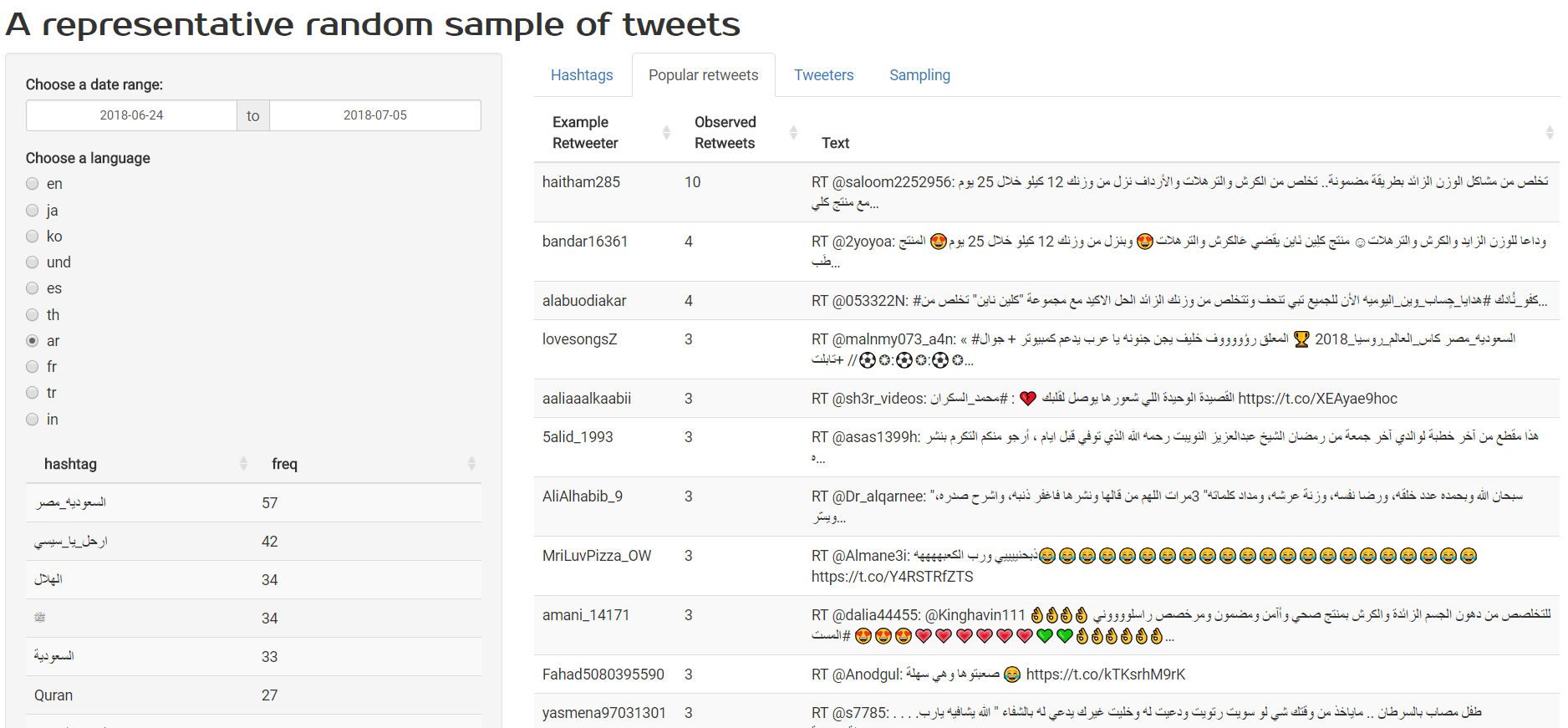
So far the main use I’ve put this data to is the Shiny app that I’ve scattered a few screenshots of in this blog post. The source code is on GitHub of course. That Shiny app writes its own SQL based on the inputs provided by the user (eg date range), queries the database and produces charts.
So what have I learned about Twitter (as opposed to about Linux administration) from the exercise? No time to explore in much depth right now, but some of the interesting things include:
- Tweets have a daily cycle, peaking at around 15:30 UTC each day (this assumes that the sampling ratio in the Twitter sample stream is roughly constant; which I think is likely as otherwise why would we see this seasonality).
- The most tweeted hashtags all relate to teen-oriented popular music. I had to look up TeenChoice just to find out what it was… My filter bubble isn’t so much a liberal-v-conservative one as something relating to different interests to most people in the world altogether. The things that dominate my own Twitter feed are not even faintly representative of Twitter as a whole (I expected this with regard to statistical computing of course, but it was interesting to find out that even US politics hardly makes a dent in the most common tweets/retweets in any particular day, compared to popular retweets such as “If the Cleveland Cavaliers win the 2018 NBA finals I’ll buy everyone who retweet’s this a jersey…” (sic) - 1.1 million retweets - and several suspiciously similar variants)
- If you ignore tweets in Japanese, Korean, Thai and Arabic script you are missing three of the top seven languages on Twitter. Any serious analysis needs to find a way to bring them on board (my first obstacle in this was getting a font that could represent as many different scripts and emojis as possible without knowing in advance the language; in the end I opted for GNU FreeFont, as described in my own answer to my question on StackOverflow about this problem)
- Only six of the ten most prolific Tweeters listed on Twitter Counter are currently prolifically tweeting. In particular, @venethis @AmexOffers @BEMANISoundTeam and @
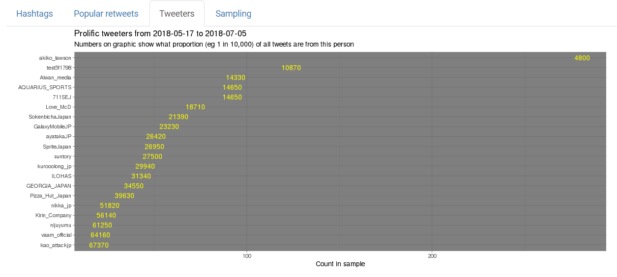
__Scc__seem to have gone either completely quiet or just much lower frequency tweeting (code for analysis). - The currently most prolific tweeter is @akiko_lawson, which I think (I don’t read Japanese) is an account associated with Lawson convenience stores. This single account issues around 1 tweet for every 5,000 tweets by anyone on the planet.
- The currently second most prolific tweeter is probably a spam bot, called @test5f1798, that amongst other things tweets pictures of Spam. Very meta.
There’s some interesting statistical challenges with using this database for inference that I might come back to. For example, I could use a small amount of auxiliary information such as the 1.1 million retweets of that Cleveland Cavaliers jersey tweet and compare it to the 105 times I found the tweet in my sample; and deduce that my sample is about 1 in 10,000 of the full population of tweets. This is consistent with the sample stream being a genuine 1% sample, of which I collect 1/120th (30 seconds every hour). So I should be able to treat my sample as a 1/12,000 sample of the whole population, clustered by the 30 second window they are in. Something for later.
