Election analysis contest entry part 2 - building the nzelect R package

Motivation

This post is the second in a series that make up my entry in Ari Lamstein’s R Election Analysis Contest, Yesterday I introduced the nzelect R package from a user perspective. Today I’m writing about how the build of that package works. This might be of interest to someone planning on doing something similar, or to anyone who wants to contribute to nzelect.

Here’s today’s themes:

Structure - separation of the preparation from the package
Modular code
Specific techniques - combining multiple CSVs, and overlaying spatial points and shapefiles

Structure

Here’s the directory structure within the Git repo that builds this package, with the individual files in the key ./prep/ folder shown on the right:

structure

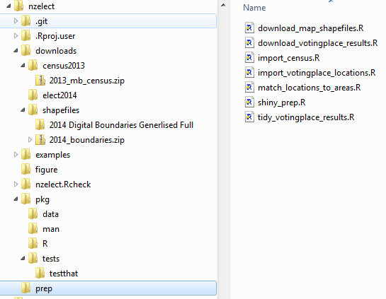
You can view, fork and clone the whole project for yourself if interested from GitHub. The code excerpts in this blog post won’t run if you just paste them into R; they need a specific folder structure that comes from running them in a clone of the main project.

Conceptually, there are three main parts of this project:

downloads and data munging that need to be done separately to the published R package, and which include products like data tidying scripts and downloaded raw data which must not be included in the package itself. This comprises the prep and downloads folders
The R package itself, which is in the pkg folder and includes subdirectories for data, man, R and tests folders
secondary material which depends on the R package being in existence and installed, such as the README for the GitHub repo, extended examples in examples including a Shiny app which will be the subject of the next post, etc.

There’s also various administrative stuff, such as the .git folder holding the version control database, .Rproj.user holding information on the RStudio project, the travis.yml file that sets up hooks from GitHub to Travis Continuous Integration, and nzelect.Rcheck holding the latest version of the R package build checks.

This is a typical structure for me. I generally don’t like an R package based in the root folder of a project. I nearly always have a bunch of stuff I want to do - prep and extended examples - that I don’t want in the built and published version of the package for end users, but I do want kept together with the code building the package in a single RStudio project and Git repository.

The project is held together by a script entitled build.R. In other projects this would make sense as a makefile but my workflow with nzelect is quite interactive (I pick and choose which files to run during development) and I’m more comfortable doing that with an R script. In principle it should work if run end to end with a fresh clone of the repository, and it looks like this:

#./build.R
# Peter Ellis, April 2016
# Builds (from scratch if necessary for a fresh clone) the nzelect R package

#----------------functionality------------
library(knitr)
library(devtools)

#-------------downloads---------------
# These are one-offs, and separated from the rest of the grooming to avoid
# repeating expensive downloads

# About 1MB worth of voting results:
source("prep/download_votingplace_results.R")

# About 130MB of shapefiles / maps, used for locating voting places in areas:
source("prep/download_map_shapefiles.R")


#----------tidying----------------
# import all the voting results CVS and amalgamate into a single object
source("prep/tidy_votingplace_results.R") # 30 seconds

# download and import the actual locations.  Includes a 575KB download.
# This script also calls ./prep/match_locations_to_areas.R from within itself 
# (takes a few minutes to run because of importing shapefiles, downloaded earlier):
source("prep/import_votingplace_locations.R") # 3 minutes

# Down the track there might be some import of economic and sociodemographic
# data here; currently only in development

# munge data for Shiny app and prompts to deploy it:
source("prep/shiny_prep.R")

#--------------build the actual package---------
# create helpfiles:
document("pkg")

# unit tests, including check against published totals
test("pkg")

# create README for GitHub repo:
knit("README.Rmd", "README.md")

# run pedantic CRAN checks
check("pkg") # currently fail due to inputenc LaTeX compile prob

# create .tar.gz for CRAN or wherever
build("pkg")

Modular code

Looking at that build.R script introduces my second theme for today - modularity. I have separate scripts for different tasks such as “download election results”, “download shapefiles” and “tidy voting place results”. This makes development easier to keep track of, and easier to run and debug a whole script at once without repeating expensive processes like downloads. Note that the downloaded data isn’t tracked by Git - that would bloat out the repository too much, so all downloads are covered in the .gitignore instead.

Some of those scripts are very short. For example, download_map_shapefiles.R is only 8 lines long including blanks:

# ./prep/download_map_shapefiles.R
# Peter Ellis, April 2016

# We want 2014 boundaries
download.file("http://www3.stats.govt.nz/digitalboundaries/annual/ESRI_Shapefile_Digital_Boundaries_2014_Generalised_12_Mile.zip",
              destfile = "downloads/shapefiles/2014_boundaries.zip", mode ="wb")

unzip("downloads/shapefiles/2014_boundaries.zip", exdir = "downloads/shapefiles")

This sort of thing is key for maintainability. If multiple people are working on a project, it also stops them treading on eachothers’ toes working on the same files at once.

Specific techniques

I won’t go through the whole project - that’s easiest done for yourself if interested from a clone of it - but will highlight three more things.

Munging the Electoral Commission CSVs

The 2014 general election results are published on the web in the form of 71 CSV files for candidate vote (one per electorate) and 71 CSV files for party vote. Each CSV has data on each voting place used by voters enrolled in the electorate (voting places are not necessarily physically in the electorate). Here’s a screenshot of a typical CSV:

csv

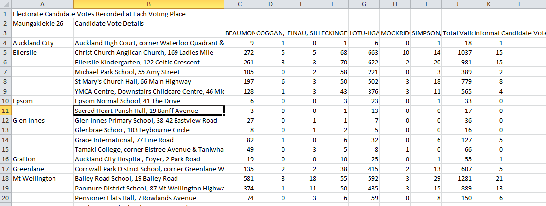
As can be seen, they go some way towards being nicely machine readable, but are not yet in tidy shape.

Some features of these CSVs include:

the name of the electorate is in cell A2
the main body of data starts in row 3
column A of the main data represents suburb, and a blank represents “same as previous entry”
the final row of the main data (not shown) is always a Total, followed by a row that is blank for columns A:E
below the main data rectangle there is a secondary rectangle of data (not shown) with data on candidates that is otherwise not presented (ie which party the candidates represent) as well as sum totals of their votes

Luckily, each CSV has an identical pattern - not identical numbers of rows and columns, but enough pattern that it is possible to programmatically identify the main data rectangle. For example, after skipping the first three rows, the next empty cell in column B indicates the main data rectangle is finished, and the row above that cell is the sum total (which needs to be excluded). Here’s the part of the tidying script that deals with those candidate CSVs:

# ./prep/tidy_votingplace_results.R
# imports previously downloaded CSVs of election results by voting place.
# So far only for 2014 General Election
# Peter Ellis, April 2016

library(tidyr)
library(dplyr)
library(stringr)

#==================2014======================================
number_electorates <- 71

#---------------------2014 candidate results-------------------
filenames <- paste0("downloads/elect2014/e9_part8_cand_", 1:number_electorates, ".csv")

results_voting_place <- list()

for (i in 1:number_electorates){
    
    # What is the electorate name?  Is in cell A2 of each csv
    electorate <- read.csv(filenames[i], skip=1, nrows=1, header=FALSE, 
                           stringsAsFactors=FALSE, fileEncoding = "UTF-8-BOM")[,1]
    
    # read in the bulk of the data
    tmp <- read.csv(filenames[i], skip=2, check.names=FALSE, 
                    stringsAsFactors=FALSE, fileEncoding = "UTF-8-BOM")
    
    # read in the candidate names and parties
    first_blank <- which(tmp[,2] == "")
    candidates_parties <- tmp[(first_blank + 2) : nrow(tmp), 1:2]
    names(candidates_parties) <- c("Candidate", "Party")
    candidates_parties <- rbind(candidates_parties,
                                data.frame(Candidate="Informal Candidate Votes", Party="Informal Candidate Votes"))
    
    # we knock out all the rows from (first_blank - 1) (which is the total)
    tmp <- tmp[-((first_blank - 1) : nrow(tmp)), ]
    names(tmp)[1:2] <- c("ApproxLocation", "VotingPlace")
    
    # in some of the data there are annoying subheadings in the second column.  We can
    # identify these as rows that return NA when you sum up where the votes should be
    tmp <- tmp[!is.na(apply(tmp[, -(1:2)], 1, function(x){sum(as.numeric(x))})), ]
    
    # need to fill in the gaps where there is no polling location
    last_ApproxLocation <- tmp[1, 1]
    for(j in 1: nrow(tmp)){
        if(tmp[j, 1] == "") {
            tmp[j, 1] <- last_ApproxLocation
        } else {
            last_ApproxLocation <- tmp[j, 1]
        }
    }  
    
    # normalise / tidy
    tmp <- tmp[names(tmp) != "Total Valid Candidate Votes"] %>%
        gather(Candidate, Votes, -ApproxLocation, -VotingPlace)
    
    tmp$Electorate <- electorate
    tmp <- tmp %>%
        left_join(candidates_parties, by = "Candidate")
    results_voting_place[[i]] <- tmp
}

# combine all electorates
candidate_results_voting_place <- do.call("rbind", results_voting_place) %>%
    mutate(Votes = as.numeric(Votes),
           Party = gsub("M..ori Party", "Maori Party", Party),
           VotingType = "Candidate")
...

Overlaying shapefiles

One important task was to take the point locations (in NZTM coordinates) of the 2,500 or so voting places and determine which meshblock, area unit, Territorial Authority and Regional Council each was in. Luckily this is a piece of cake with the over() function from the sp package. The process is:

import a shapefile of the boundaries we want (the originals are at http://www.stats.govt.nz/browse_for_stats/Maps_and_geography/Geographic-areas/digital-boundary-files.aspx and a script in the project downloads the versions for 2014) into R as a sp::SpatialPolygonsDataFrame object
use the proj4string from that shapefile to help convert the NZTM coordinates into a sp::SpatialPoints object
use sp::over() to map the SpatialPoints to the SpatialPolygonsDataFrame.

# ./prep/match_locations_to_areas.R
# Peter Ellis, April 2016

# depends on the shapefiles having already been downloaded from
# ./prep/download_map_shapefiles.R; and Locations2014 to have
# been created via .prep/import_votingplace_locations.R
# This script then matches those point locations with the polygons
# of Regional Councils, Territorial Authority, and Area Unit.

# This script is called from ./prep/import_votingplace_locations.R
library(rgdal)

#-------------Import Territorial Authority map------------------
TA <- readOGR("downloads/shapefiles/2014 Digital Boundaries Generlised Full",
              "TA2014_GV_Full")

#------------------convert locations to sp format-----------
locs <- SpatialPoints(coords = Locations2014[, c("NZTM2000Easting", "NZTM2000Northing")],
                      proj4string = TA@proj4string)

#-------------Match to Territorial Authority-------
locs2 <- over(locs, TA)
Locations2014$TA2014_NAM <- locs2$TA2014_NAM
..

Unit tests

Any serious coding project needs unit tests so you can be sure that things, once fixed, continue to work as you make changes to other parts of the project. This applies as much to analytical projects as to software development. Hadley Wickham’s testthat package gives a nice structure for including unit tests in the actual check and build of an R package, and I use that in this project. Here’s some of the tests I’m using, in the ./pkg/tests/testthat/ directory:

require(testthat)
require(dplyr)

# Must match results from 
# http://www.electionresults.govt.nz/electionresults_2014/e9/html/e9_part1.html

# absolute numbers
expect_that(
    sum(filter(GE2014, Party == "National Party" & VotingType == "Party")$Votes),
    equals(1131501)
)

expect_that(
    sum(filter(GE2014, Party == "National Party" & VotingType == "Candidate")$Votes),
    equals(1081787)
)

expect_that(
    sum(filter(GE2014, Party == "Labour Party" & VotingType == "Party")$Votes),
    equals(604535)
)

expect_that(
    sum(filter(GE2014, Party == "Labour Party" & VotingType == "Candidate")$Votes),
    equals(801287)
)

expect_that(
    sum(filter(GE2014, Party == "New Zealand First Party" & VotingType == "Party")$Votes),
    equals(208300)
)

expect_that(
    sum(filter(GE2014, Party == "New Zealand First Party" & VotingType == "Candidate")$Votes),
    equals(73384)
)

expect_that(
    sum(filter(GE2014, Party == "Patriotic Revolutionary Front" & VotingType == "Candidate")$Votes),
    equals(48)
)

# percentages
expect_that(
    round(sum(filter(GE2014, Party == "National Party" & VotingType == "Party")$Votes) /
        sum(filter(GE2014, VotingType == "Party" & Party != "Informal Party Votes")$Votes) * 100, 2),
    equals(47.04)
 )


expect_that(
    round(sum(filter(GE2014, Party == "Green Party" & VotingType == "Candidate")$Votes) /
              sum(filter(GE2014, VotingType == "Candidate" & Party != "Informal Candidate Votes")$Votes) * 100, 2),
    equals(7.06)
)

# compare to http://www.electionresults.govt.nz/electionresults_2014/electorate-47.html

rotorua <- GE2014 %>%
    filter(Electorate == "Rotorua 47" & VotingType == "Candidate") %>%
    group_by(Candidate) %>%
    summarise(Votes = sum(Votes)) %>%
    arrange(desc(Votes))

expect_that(
    tolower(as.character(rotorua[1, 1])),
    equals(tolower("McClay, Todd Michael"))
)

expect_that(
    as.numeric(rotorua[1, 2]),
    equals(18715)
)

expect_that(
    tolower(as.character(rotorua[6, 1])),
    equals(tolower("russell, lyall"))
)

expect_that(
    as.numeric(rotorua[6, 2]),
    equals(132)
)

Conclusion

The three themes for today:

structure - separating prep, package, and extended use
modularity
a few specific techniques of data cleaning

That’s enough for now. Stay tuned for the next post in the series, which looks at the Shiny app I built as an extended example of use of the nzelect package.