In the last few years there have been more attempts at a fresh approach to statistical timeseries forecasting using the increasingly accessible tools of machine learning. This means methods like neural networks and extreme gradient boosting, as supplements or even replacements of the more traditional tools like auto-regressive integrated moving average (ARIMA) models.
As an example aiming to get these methods into accessible production, Rob Hyndman’s forecast R package now includes the nnetar function. This takes lagged versions of the target variable as inputs and uses a neural network with a single hidden layer to model the results. Forecasting is then done one period at a time, with each new period then becoming part of the matrix of explanatory variables for the subsequent periods. All this is put into play (from the user’s perspective) with one or two lines of easily understood code.
I’ve started on an R package forecastxgb which will adapt this approach to extreme gradient boosting, popularly implemented by the astonishingly fast and effective xgboost algorithm. xgboost has become dominant in parts of the predictive analytics field, particularly through competitions such as those hosted by Kaggle. From the forecastxgb vignette:
The
forecastxgbpackage aims to provide time series modelling and forecasting functions that combine the machine learning approach of Chen, He and Benesty’sxgboostwith the convenient handling of time series and familiar API of Rob Hyndman’sforecast. It applies to time series the Extreme Gradient Boosting proposed in Greedy Function Approximation: A Gradient Boosting Machine, by Jerome Friedman in 2001. xgboost has become an important machine learning algorithm; nicely explained in this accessible documentation.
My aim is to make the data handling - creating all those lagged variables, and lagged versions of the xreg variables, and dummies for seasons - easy, and to make the API familiar to timeseries analysts familiar with the forecast package. Usage is straightforward, as shown here modelling Australia’s quarterly gas production using the gas time series included with forecast:
devtools::install_github("ellisp/forecastxgb-r-package/pkg") # CRAN release still to come
library(forecastxgb)
model <- xgbts(gas)
fc <- forecast(model, h = 12)
plot(fc)
[results not shown but will look familiar to anyone using the forecast toolkit]
I’m hoping that at least a few people will try it out and give me feedback before I feel comfortable publishing it on CRAN.
The vignette has more examples, including with external regressors via the xreg= argument. This is where I think the approach might have something to offer that is competitive with traditional techniques, but I’m still on the lookout for a ready-to-go mass collection of data with x regressors, set up like a forecasting competition (ie with the actual results for assessment), to test it against.
Here is an extended univariate test of my new xgbts function against nnetar and two more traditional time series methods - ARIMA and the Theta method. Because it is well known that forecasting is more successful when averages of several forecasts are used, I also look at all the combinations of the four models, meaning there are 15 different sets of forecasts in the end for each data series. I test the approach on the 1,311 data series from the 2010 Tourism forecasting competition conveniently available in the Tcomp R package which I released and blogged about a few weeks ago. The chart below shows mean absolute scaled error (MASE) of the various models’ forecasts when confronted with the actual results.
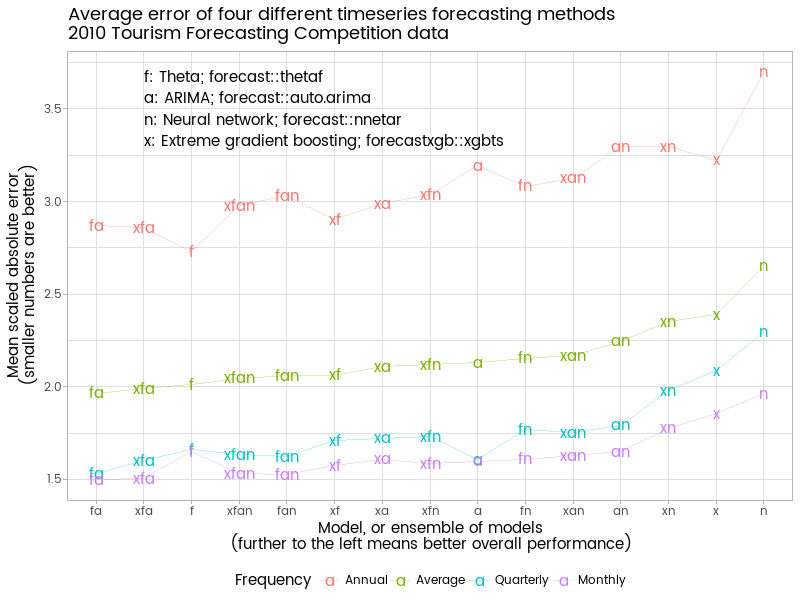
We see the overall best performing ensemble is the average of the Theta and ARIMA models - the two from the more traditional timeseries forecasting approach. The two machine learning methods (neural network and extreme gradient boosting) are not as effective, at least in these implementations. As individual methods, they are the two weakest, although the extreme gradient boosting method provided in forecastxgb performs noticeably better than forecast::nnetar (with this particular set of data - as I write, my computer finishes churning through all 3,000+ M3 competition datasets, which goes the other way in terms of xgbts versus nnetar).
Theta by itself is the best performing with the annual data - simple methods work well when the dataset is small and highly aggregate. The best that can be said of the xgbts approach in this context is that it doesn’t damage the Theta method much when included in a combination - several of the better performing ensembles have xgbts as one of their members. In contrast, the neural network models do badly with this particular collection of annual data.
Adding auto.arima and xgbts to an ensemble of quarterly or monthly data definitely improves on Theta by itself. The best performing single model for quarterly or monthly data is auto.arima followed by thetaf. Again, neural networks are the poorest of the four individual models.
Overall, I conclude that with this sort of univariate data, xgbts with its current default settings has little to add to an ensemble that already contains auto.arima and thetaf (or - not shown - the closely related ets). It’s likely that more investigation will show differing results with differing defaults, particuarly of the maximum number of lags to use. It’s also possible that inclusion of xreg external regressors might shift the balance in favour of xgbts and maybe even nnetar - the more complex and larger the dataset, the better the chance that these methods will have something to offer. Watch this space. Any ideas welcomed. Specific bugs, suggestions or enhancement requests are particularly welcome on the forecastxgb page on GitHub.
Here’s the code that did that test against the tourism competition data:
#=============prep======================
library(Tcomp)
library(foreach)
library(doParallel)
library(forecastxgb)
library(dplyr)
library(ggplot2)
library(scales)
library(Mcomp)
#============set up cluster for parallel computing===========
cluster <- makeCluster(7) # only any good if you have at least 7 processors :)
registerDoParallel(cluster)

clusterEvalQ(cluster, {
   library(Tcomp)
   library(forecastxgb)
   library(Mcomp)
})


#===============the actual analytical function==============
competition <- function(collection, maxfors = length(collection)){
   if(class(collection) != "Mcomp"){
      stop("This function only works on objects of class Mcomp, eg from the Mcomp or Tcomp packages.")
   }
   nseries <- length(collection)
   mases <- foreach(i = 1:maxfors, .combine = "rbind") %dopar% {
      thedata <- collection[[i]]
      mod1 <- xgbts(thedata$x)
      fc1 <- forecast(mod1, h = thedata$h)
      fc2 <- thetaf(thedata$x, h = thedata$h)
      fc3 <- forecast(auto.arima(thedata$x), h = thedata$h)
      fc4 <- forecast(nnetar(thedata$x), h = thedata$h)
      # copy the skeleton of fc1 over for ensembles:
      fc12 <- fc13 <- fc14 <- fc23 <- fc24 <- fc34 <- fc123 <- fc124 <- fc134 <- fc234 <- fc1234 <- fc1
      # replace the point forecasts with averages of member forecasts:
      fc12$mean <- (fc1$mean + fc2$mean) / 2
      fc13$mean <- (fc1$mean + fc3$mean) / 2
      fc14$mean <- (fc1$mean + fc4$mean) / 2
      fc23$mean <- (fc2$mean + fc3$mean) / 2
      fc24$mean <- (fc2$mean + fc4$mean) / 2
      fc34$mean <- (fc3$mean + fc4$mean) / 2
      fc123$mean <- (fc1$mean + fc2$mean + fc3$mean) / 3
      fc124$mean <- (fc1$mean + fc2$mean + fc4$mean) / 3
      fc134$mean <- (fc1$mean + fc3$mean + fc4$mean) / 3
      fc234$mean <- (fc2$mean + fc3$mean + fc4$mean) / 3
      fc1234$mean <- (fc1$mean + fc2$mean + fc3$mean + fc4$mean) / 4
      mase <- c(accuracy(fc1, thedata$xx)[2, 6],
                accuracy(fc2, thedata$xx)[2, 6],
                accuracy(fc3, thedata$xx)[2, 6],
                accuracy(fc4, thedata$xx)[2, 6],
                accuracy(fc12, thedata$xx)[2, 6],
                accuracy(fc13, thedata$xx)[2, 6],
                accuracy(fc14, thedata$xx)[2, 6],
                accuracy(fc23, thedata$xx)[2, 6],
                accuracy(fc24, thedata$xx)[2, 6],
                accuracy(fc34, thedata$xx)[2, 6],
                accuracy(fc123, thedata$xx)[2, 6],
                accuracy(fc124, thedata$xx)[2, 6],
                accuracy(fc134, thedata$xx)[2, 6],
                accuracy(fc234, thedata$xx)[2, 6],
                accuracy(fc1234, thedata$xx)[2, 6])
      mase
   }
   message("Finished fitting models")
   colnames(mases) <- c("x", "f", "a", "n", "xf", "xa", "xn", "fa", "fn", "an",
                        "xfa", "xfn", "xan", "fan", "xfan")
   return(mases)
}


## Test on a small set of data, useful during dev
small_collection <- list(tourism[[1]], tourism[[2]], tourism[[3]], tourism[[4]], tourism[[5]], tourism[[6]])
class(small_collection) <- "Mcomp"
test1 <- competition(small_collection)


#========Fit models==============
system.time(t1  <- competition(subset(tourism, "yearly")))
system.time(t4 <- competition(subset(tourism, "quarterly")))
system.time(t12 <- competition(subset(tourism, "monthly")))

# shut down cluster to avoid any mess:
stopCluster(cluster)


#==============present tourism results================
results <- c(apply(t1, 2, mean),
             apply(t4, 2, mean),
             apply(t12, 2, mean))

results_df <- data.frame(MASE = results)
results_df$model <- as.character(names(results))
periods <- c("Annual", "Quarterly", "Monthly")
results_df$Frequency <- rep.int(periods, times = c(15, 15, 15))

best <- results_df %>%
   group_by(model) %>%
   summarise(MASE = mean(MASE)) %>%
   arrange(MASE) %>%
   mutate(Frequency = "Average")

Tcomp_results <- results_df %>%
   rbind(best) %>%
   mutate(model = factor(model, levels = best$model)) %>%
   mutate(Frequency = factor(Frequency, levels = c("Annual", "Average", "Quarterly", "Monthly")))

leg <- "f: Theta; forecast::thetaf\na: ARIMA; forecast::auto.arima
n: Neural network; forecast::nnetar\nx: Extreme gradient boosting; forecastxgb::xgbts"

Tcomp_results %>%
   ggplot(aes(x = model, y =  MASE, colour = Frequency, label = model)) +
   geom_text(size = 6) +
   geom_line(aes(x = as.numeric(model)), alpha = 0.25) +
   scale_y_continuous("Mean scaled absolute error\n(smaller numbers are better)") +
   annotate("text", x = 2, y = 3.5, label = leg, hjust = 0) +
   ggtitle("Average error of four different timeseries forecasting methods\n2010 Tourism Forecasting Competition data") +
   labs(x = "Model, or ensemble of models\n(further to the left means better overall performance)")